Draft pod pairings Pt 2 - Taking account of luck

In my previous post, I pondered about the single elimination tournmanets (such as those in side events at a MagicFest) and whether I wanted to face my friend in the first round or in the final round to maximize winnings assuming we pooled our winnings. In that post, I considered two cases:

• 1) where the game being played is just a coin flip
• 2) where the game being played is a complete game of skill and the better player wins 100% of the time.

The results were intuitive. If the game was a coin flip, then our winnings are the same regardless of when or if we played against each other. If the game was a pure game of skill then a pair of better than average players would prefer to play each other in the final round, while a pair of worse than average players would want to play each other in the first round to guarantee a free win.

However, the game I’m considering is Magic: The Gathering, a game with a long history of games being decided with lucky draws even in the professional level. It has been argued that Magic’s randomness has contributed to its longevity, by allowing newer players and people of lesser skill to be able to get wins against better players and not feel bad all the time¹. So the true win rate of better players is somewhere in between a pure coin flip and 100% certainty.

even a hall of famer can’t escape losing to a lucky topdeck. or perhaps brian kibler just wanted the other guy to not feel bad.

I’ll use the same settings as the previous post. The tournament is a 8 person single-elimination tournament. The prizing structure is 0 tickets for 0 wins, 20 tickets for 1 win, 200 tickets for 2 wins, and 400 tickets for 3 wins. All players have a skill value in $[0, 1]$. I have skill $x$, my friend Jon has skill $y$. All other players have skills randomly chosen uniformly over the range of $[0, 1]$. Again for simplicity, let’s assume that $x > y$. But everything that follows can be flipped to get the case where $y > x$ ².

The addition from the previous post’s model is that I’m adding a constant $p$ that represents the probability that the player with higher skill beats the player with lower skill. So it’s still mostly a game of skill, but lower skilled players can steal a win $(1-p)$ % of the time. The 2 cases from the previous post map to the cases where $p = 0.5$ (coin flip) and $p = 1.0$ (pure skill). I’m only considering $p$ in the range of $[0.5, 1.0]$. Values of $p$ less than $0.5$ would mean the game favors the “worse” players, so it’s basically the same as redefining “worse” as “better”.

The addition of $p$ complicates the probability calculations a bit. Instead of expanding and calculating all the probabilities directly, I’ll build up from smaller parts to build up the full calculations.

Let’s imagine I just won a game. My next opponent must then be also be a winner of some other game. Let $Z_{winner}$ be my next opponent’s skill rating and $Z_a$ and $Z_b$ be the skill levels of the 2 players of the game that my next opponent just won (Note: $Z_{winner}$ is either $Z_a$ or $Z_b$ because the winner is one of the 2 players). What is the probability that $Z_{winner}$ is greater than some value $t$?

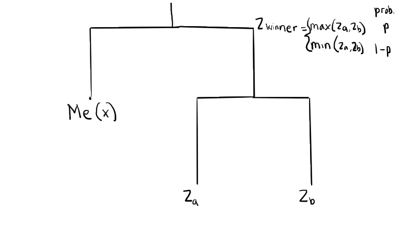
With probability $p$, $Z_{winner}$ is $max(Z_a, Z_b)$. What is the probability that $max(Z_a, Z_b) < t$? $Z_a$ and $Z_b$ are independent³ , so

$$\begin{align*} P(max(Z_a, Z_b) < t) &= P(Z_a < t\text{ and }Z_b < t) \\ &= P(Z_a < t)P(Z_b < t) \end{align*}$$

I also used similar logic in the previous post. But then I immediately reduced this by noting $P(Z_0 < t) = t$ for the uniformly random players, so I got that my second round opponent’s skill rating is less than $t$ with probability $t^2$. Here it’s useful for me to keep this formula generic to plug in different distributions of individual players as needed.

Here’s a more functional way to express the formula.

$$\text{cdf_max}(\text{cdf_a}, \text{cdf_b}) = \text{cdf_a} * \text{cdf_b}$$

Here I use the term $cdf$ as shorthand for cumulative distribution function to represent a function for the random value being less than some value $t$.

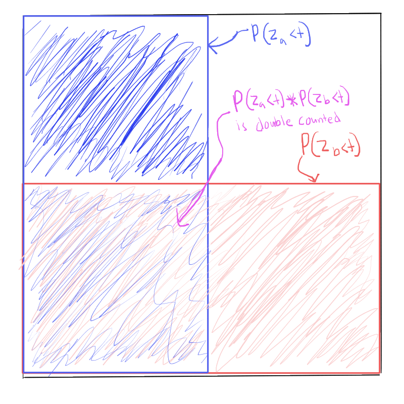
With probability $1-p$, $Z_{winner}$ is actually the lower player’s skill value which is $min(Z_a, Z_b)$ instead. What is the probability that $min(Z_a, Z_b) < t$? It’s the probability that either $Z_a < t$ or $Z_b < t$. We can add $P(Z_a < t)$ and $P(Z_b < t)$ to get the sum of probabilities that either is less than $t$, but then we would be double-counting the instances where both $Z_a$ and $Z_b$ are less than $t$ at the same time. We account for the double-counting by subtracting one instance of $P(Z_a < t)*P(Z_b < t)$ ³.

$$\begin{align*} P(min(Z_a, Z_b) < t) &= P(Z_a < t\text{ or }Z_b < t) \\ &= P(Z_a < t) + P(Z_b < t) - P(Z_a < t)* P(Z_b < t) \end{align*}$$

Expressed in a functional form:

$$\text{cdf_min}(\text{cdf_a}, \text{cdf_b}) = \text{cdf_a} + \text{cdf_b} - \text{cdf_a}*\text{cdf_b}$$

Overall, we can express the probability of $Z_\text{winner}$ being less than $t$ as this function:

$$\text{cdf_winner}(\text{cdf_a}, \text{cdf_b}, p) = p * \text{cdf_max}(\text{cdf_a}, \text{cdf_b}) + (1-p)*\text{cdf_min}(\text{cdf_a}, \text{cdf_b})$$

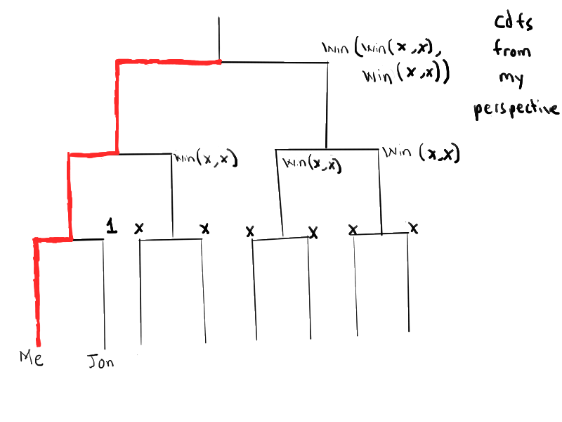
So we can express the distribution of a winner’s skill of a game based on the distribution of the 2 individual player’s skills. But what is is $\text{cdf_a}$ and $\text{cdf_b}$? At the initial selection of random players, each player is chosen uniformly in the spectrum of $[0, 1]$, so $\text{cdf_a} = t$ in this case. If the player is Jon, then $Z_a$ is known to be $y$, $\text{cdf_a}$ is 1 if $y > t$ and 0 otherwise. From these base values and a function to calculate the distribution of the winner of a any game, we can calculate all the probabilities we need for the tournament.

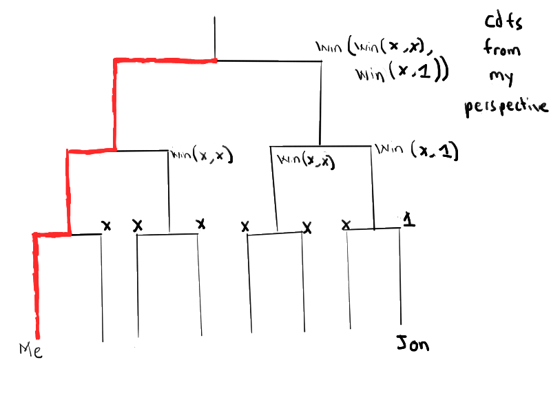
For example, consider the case where Jon and I face each other in the first round. My first round opponent is Jon, who I know I have higher skill rating over. The second round opponent would be a winner of 2 random players. The third round opponent is a winner of 2 people that won over random players themselves. Plugging those values into the $\text{cdf_winner}$ function (in some cases many times) gives us the distribution of player skill’s over every round.

My perspective, matched with Jon in first round $\begin{align*} &\text{p_opp_1_less_than_x} = P(\text{I am better than first opponent}) = 1 \\ &\text{p_opp_2_less_than_x} = P(\text{I am better than second opponent}) = \text{cdf_winner}(x, x, p) \\ &\text{p_opp_3_less_than_x} = P(\text{I am better than third opponent}) = \text{cdf_winner}(\text{cdf_winner}(x, x, p), \text{cdf_winner}(x, x, p), p) \end{align*}$

Using these player skill distributions in each round, we can calculate my expected winnings in the tournament.

$$\begin{alignat}{2} &\text{p_win_game_1} = P(\text{I win first game}) &&= \text{p_opp_1_less_than_x} * p + (1 - \text{p_opp_1_less_than_x}) * (1-p) \\ &\text{p_win_game_2} = P(\text{I win second game}) &&= \text{p_opp_2_less_than_x} * p + (1 - \text{p_opp_2_less_than_x}) * (1-p) \\ &\text{p_win_game_3} = P(\text{I win third game}) &&= \text{p_opp_3_less_than_x} * p + (1 - \text{p_opp_3_less_than_x}) * (1-p) \end{alignat}$$ $$\begin{align*} \text{Expected tickets} &= (1 - \text{p_win_game_1}) * 0 \\ &+ \text{p_win_game_1} * (1 - \text{p_win_game_2}) * 20 \\ &+ \text{p_win_game_1} * \text{p_win_game_2} * (1 - \text{p_win_game_3}) * 200 \\ &+ \text{p_win_game_1} * \text{p_win_game_2} * \text{p_win_game_3} * 400 \end{align*}$$

Similarly, we can calculate the distributions for Jon’s opponents skill. I’ll leave out the derivations for probabilities of winning the first, second, and third games and expected tickets because the calculations are very similar.

Jon’s perspective, matched with me in first round $\begin{align*} &\text{p_opp_1_less_than_y} = 0 \\ &\text{p_opp_2_less_than_y} = \text{cdf_winner}(y, y, p) \\ &\text{p_opp_3_less_than_y} = \text{cdf_winner}(\text{cdf_winner}(y, y, p), \text{cdf_winner}(y, y, p), p) \end{align*}$

In the case of Jon and I being seeded in different sides of the tournament, the formulas for opponent skill distributions are similar. We replace the first opponent with a random player, and then insert Jon (or myself) as a possible opponent instead of a random player in the third round.

My perspective, playing Jon only possibly in final round $\begin{align*} &\text{p_opp_1_less_than_x} = x \\ &\text{p_opp_2_less_than_x} = \text{cdf_winner}(x, x, p) \\ &\text{p_opp_3_less_than_x} = \text{cdf_winner}(\text{cdf_winner}(x, 1, p), \text{cdf_winner}(x, x, p), p) \end{align*}$

Jon’s perspective, playing me only possibly in final round $\begin{align*} &\text{p_opp_1_less_than_y} = y \\ &\text{p_opp_2_less_than_y} = \text{cdf_winner}(y, y, p) \\ &\text{p_opp_3_less_than_y} = \text{cdf_winner}(\text{cdf_winner}(y, 0, p), \text{cdf_winner}(y, y, p), p) \end{align*}$

So we can expand all of these formulas and get all of the expected winnings. That’s way too many terms to expand algebraically though, so I just wrote a program instead to calculate expected winnings over values given $x$, $y$, and $p$. Similar to the previous post, I’ll graph out the preference of being matched up in the first round vs. the final round, but I added different colors to show the change of degree of preference to get an idea of how the curve moves.

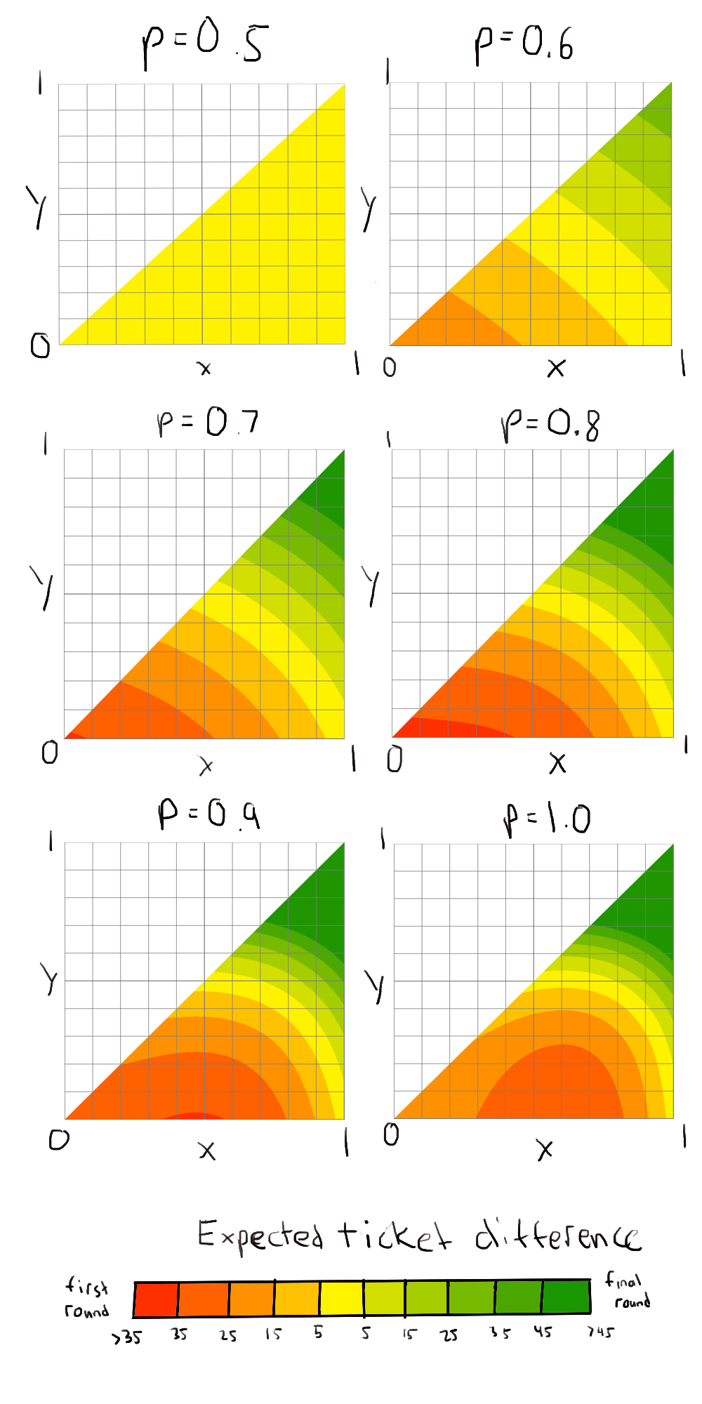
Intuitively, as p goes from $0.5$ to $1.0$, the graphs go from all outcomes being the same to a clear preference for one pairing over the other. The region around $(1, 1)$ increasingly prefers a final round pairing as $p$ goes up. However, the region that most prefers the first round pairing interestingly starts moving to the right, as if it were an eye of a storm moving along the triangle ⁴, a hurricane search for free wins.

Interestingly, the corner of $(0, 0)$ doesn’t increasingly prefer the free win as $p$ gets closer to $1$. Clearly this corner overall prefers $p$ to be equal to $0.5$ overall to make up for the lack of skill. The preference for pairing in the first round comes from wanting a free win to possibly luckily spike up to the third round to get much more tickets. But as $p$ gets closer to $1$, the possibility of winning future rounds becomes vanishingly low so the expected ticket difference approaches the single win prize of just 20 tickets.

So the conclusion remains the same even when the game isn’t a pure game of luck or skill. A pair of really bad players still prefer to take the free win by matching in the first round, a pair of really good players still prefer to split up to get maximum winnings, and there’s still a range where a good player and a bad player may still want to match up with each other to hand the better player a free win in order to maximize overall winnings. The value of $p$ mostly just makes the preference much more clear, or moves the preference maximizer around the triangle.

Now this model is still pretty simple, even though it results in a mess of formulas. I could have used a win model that takes into account the degree of skill disparity. That is, use a model such that players of similar skill will still have relatively even chances of winning vs. a player of much higher skill winning perhaps 99% of the time against a much lower skill player. Most models of player rating do this, such as Elo rating and its variants. I decided against it because it complicates the modeling even further, and would require me to choose even more parameters than just the one parameter $p$ I had while having no data to fit it on! I doubt it would change anything, but if anyone wants to take a stab at it, I’m happy to see those results.

Footnotes:

1. Like Jon was in the previous post. In this post, he will get his vengeance and be allowed to win some games against me. I would be glad to give him some wins if it makes him feel better. ↩

2. I realize that I’m leaving out the case $x = y$, but I don’t want to deal with writing $\leq$ symbols. I’m sure it doesn’t really matter due to some “measure-zero” thing, but my math skills aren’t so good that I can say that with a straight face. Besides, Jon and I can’t possibly have the same skill level, we’re different people after all. ↩

3. See Inclusion-Exclusion Principle. This principle extends to counting events over many different levels of overlaps. ↩ ↩²

4. As a curiosity, I looked at the minimizer of the expected ticket difference as $p$ goes from $0$ to $1$. Visually, the minimizer starts from $(0, 0)$ when $p$ is around $0.5$. When $p = 1$, we get the formula from the first post that the difference is $y * (20 + 180 y^2) - (1-x)*(20 + 180 x^2)$. In the range we’re considering, this is minimized when $y = 0$ and $(1-x)*(20 + 180 x^2)$ is maximized in respect to $x$ in the range of $[0, 1]$. The value of $x$ that maximizes that is $(1+\sqrt{2/3})/3 \approx {0.605}$. So the hurricane moves from $(0, 0)$ to $(0.605, 0)$ as $p$ goes from $0$ to $1$. ↩